User:Manudouz/sandbox/Complete-linkage clustering
Working example
[edit]This working example is based on a JC69 genetic distance matrix computed from the 5S ribosomal RNA sequence alignment of five bacteria: Bacillus subtilis (), Bacillus stearothermophilus (), Lactobacillus viridescens (), Acholeplasma modicum (), and Micrococcus luteus ().[1][2]
First step
[edit]- First clustering
Let us assume that we have five elements and the following matrix of pairwise distances between them:
| a | b | c | d | e | |
|---|---|---|---|---|---|
| a | 0 | 17 | 21 | 31 | 23 |
| b | 17 | 0 | 30 | 34 | 21 |
| c | 21 | 30 | 0 | 28 | 39 |
| d | 31 | 34 | 28 | 0 | 43 |
| e | 23 | 21 | 39 | 43 | 0 |
In this example, is the smallest value of , so we join elements and .
- First branch length estimation
Let denote the node to which and are now connected. Setting ensures that elements and are equidistant from . This corresponds to the expectation of the ultrametricity hypothesis. The branches joining and to then have lengths (see the final dendrogram)
- First distance matrix update
We then proceed to update the initial proximity matrix into a new proximity matrix (see below), reduced in size by one row and one column because of the clustering of with . Bold values in correspond to the new distances, calculated by retaining the maximum distance between each element of the first cluster and each of the remaining elements:
Italicized values in are not affected by the matrix update as they correspond to distances between elements not involved in the first cluster.
Second step
[edit]- Second clustering
We now reiterate the three previous steps, starting from the new distance matrix :
| (a,b) | c | d | e | |
|---|---|---|---|---|
| (a,b) | 0 | 30 | 34 | 23 |
| c | 30 | 0 | 28 | 39 |
| d | 34 | 28 | 0 | 43 |
| e | 23 | 39 | 43 | 0 |
Here, is the lowest value of , so we join cluster with element .
- Second branch length estimation
Let denote the node to which and are now connected. Because of the ultrametricity constraint, the branches joining or to , and to , are equal and have the following total length:
We deduce the missing branch length: (see the final dendrogram)
- Second distance matrix update
We then proceed to update the matrix into a new distance matrix (see below), reduced in size by one row and one column because of the clustering of with :
Third step
[edit]- Third clustering
We again reiterate the three previous steps, starting from the updated distance matrix .
| ((a,b),e) | c | d | |
|---|---|---|---|
| ((a,b),e) | 0 | 39 | 43 |
| c | 39 | 0 | 28 |
| d | 43 | 28 | 0 |
Here, is the smallest value of , so we join elements and .
- Third branch length estimation
Let denote the node to which and are now connected. The branches joining and to then have lengths (see the final dendrogram)
- Third distance matrix update
There is a single entry to update:
Final step
[edit]The final matrix is:
| ((a,b),e) | (c,d) | |
|---|---|---|
| ((a,b),e) | 0 | 43 |
| (c,d) | 43 | 0 |
So we join clusters and .
Let denote the (root) node to which and are now connected. The branches joining and to then have lengths:
We deduce the two remaining branch lengths:
The complete-linkage dendrogram
[edit]

The dendrogram is now complete. It is ultrametric because all tips ( to ) are equidistant from :
The dendrogram is therefore rooted by , its deepest node.
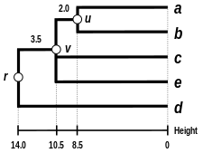
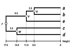
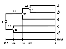
Comparison of clustering methods
[edit] |

|
 |
 |
| Single-linkage clustering | Complete-linkage clustering | WPGMA | UPGMA |
- ^ Erdmann, Volker A.; Wolters, Jörn (1986). "Collection of published 5S, 5.8S and 4.5S ribosomal RNA sequences". Nucleic Acids Research. 14 (Suppl): r1–r59. ISSN 0305-1048. PMC 341310. PMID 2422630.
{{cite journal}}: CS1 maint: PMC format (link) - ^ Olsen, G. J. (1988). "Phylogenetic analysis using ribosomal RNA". Methods in Enzymology. 164: 793–812. ISSN 0076-6879. PMID 3241556.


