Edgeworth box

In economics, an Edgeworth box, sometimes referred to as an Edgeworth-Bowley box, is a graphical representation of a market with just two commodities, X and Y, and two consumers. The dimensions of the box are the total quantities Ωx and Ωy of the two goods.
Let the consumers be Octavio and Abby. The top right-hand corner of the box represents the allocation in which Octavio holds all the goods, while the bottom left corresponds to complete ownership by Abby. Points within the box represent ways of allocating the goods between the two consumers.
Market behaviour will be determined by the consumers' indifference curves. The blue curves in the diagram represent indifference curves for Octavio, and are shown as convex from his viewpoint (i.e. seen from the bottom left). The orange curves apply to Abby, and are convex as seen from the top right. Moving up and to the right increases Octavio's allocation and puts him onto a more desirable indifference curve while placing Abby onto a less desirable one.
Convex indifference curves are considered to be the usual case. They correspond to diminishing returns for each good relative to the other.
Exchange within the market starts from an initial allocation known as an endowment.
The main use of the Edgeworth box is to introduce topics in general equilibrium theory in a form in which properties can be visualised graphically. It can also show the difficulty of moving to an efficient outcome in the presence of bilateral monopoly.[1] In the latter case, it serves as a precursor to the bargaining problem of game theory that allows a unique numerical solution.[2][3]
History
[edit]Development of the Edgeworth box
[edit]The Edgeworth box is named after Francis Ysidro Edgeworth,[4] who presented it in his book Mathematical Psychics: An Essay on the Application of Mathematics to the Moral Sciences, 1881.[5] Edgeworth's original two-axis depiction was developed into the now familiar box diagram by Pareto in his 1906 Manual of Political Economy and was popularized in a later exposition by Bowley. The modern version of the diagram is commonly referred to as the Edgeworth–Bowley box.[6]
The mathematical theory of economic equilibrium
[edit]The conceptual framework of equilibrium in a market economy was developed by Léon Walras[7] and further extended by Vilfredo Pareto.[8] It was examined with close attention to generality and rigour by twentieth century mathematical economists including Abraham Wald,[9] Paul Samuelson,[10] Kenneth Arrow and Gérard Debreu.[11] This was part of a wider movement in which Wald also sought to bring greater rigour to decision theory and many mathematicians concentrated on minimising dependence on the axiom of choice.
The theory of Walrasian markets has taken pains to find the most general premises from which a given conclusion can be obtained. Areas in which premises can be strengthened or weakened include:
- Whether functions are differentiable;
- Whether indifference curves are primitive or derivable from utility functions; and
- Whether indifference curves are convex.
Assumptions are also made of a more technical nature, e.g. non-reversibility, saturation, etc.
The pursuit of rigour is not always conducive to intelligibility. In this article indifference curves will be treated as primitive. At first we will view them as convex and differentiable and concentrate on interior equilibria, but we will subsequently relax these assumptions.
Market equilibrium
[edit]
Since there are only two commodities the effective price is the exchange rate between them. Our aim is to find the price at which market equilibrium can be attained, which will be a point at which no further transactions are desired, starting from a given endowment. These quantities will be determined by the indifference curves of the two consumers as shown in Fig. 2.
We shall assume that every day Octavio and Abby go to market with endowments (ωx,ωy ) and (Ωx – ωx , Ωy – ωy ) of the two commodities, corresponding to the position ω in the diagram. The two consumers will exchange between themselves under competitive market behaviour. This assumption requires a certain suspension of disbelief since the conditions for perfect competition – which include an infinite number of consumers – aren't satisfied.
If two X's exchange for a single Y, then Octavio's and Abby's transaction will take them to some point along the solid grey line, which is known as a budget line. (To be more precise, a budget line may be defined as a straight line through the endowment point representing allocations obtainable by exchange at a certain price.) Budget lines for a couple of other prices are also shown as dashed and dotted lines in Fig. 2.
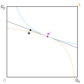
The equilibrium corresponding to a given endowment ω is determined by the pair of indifference curves which have a common tangent such that this tangent passes through ω. We will use the term 'price line' to denote a common tangent to two indifference curves. An equilibrium therefore corresponds to a budget line which is also a price line, and the price at equilibrium is the gradient of the line. In Fig. 3 ω is the endowment and ω' is the equilibrium allocation.
The reasoning behind this is as follows.

Firstly, any point in the box must lie on exactly one of Abby's indifference curves and on exactly one of Octavio's. If the curves cross (as shown in Fig. 4) then they divide the immediate neighbourhood into four regions, one of which (shown as pale green) is preferable for both consumers; therefore a point at which indifference curves cross cannot be an equilibrium, and an equilibrium must be a point of tangency.
Secondly, the only price which can hold in the market at the point of tangency is the one given by the gradient of the tangent, since at only this price will the consumers be willing to accept limitingly small exchanges.
And thirdly (the most difficult point) all exchanges taking the consumers on the path from ω to equilibrium must take place at the same price. If this is accepted, then that price must be the one operative at the point of tangency, and the result follows.
In a two-person economy there is no guarantee that all exchanges will take place at the same price. But the purpose of the Edgeworth box is not to illustrate the price fixing which can take place when there is no competition, but rather to illustrate a competitive economy in a minimal case. So we may imagine that instead of a single Abby and a single Octavio we have an infinite number of clones of each, all coming to market with identical endowments at different times and negotiating their way gradually to equilibrium. A newly arrived Octavio may exchange at market price with an Abby who is close to equilibrium, and so long as a newly arrived Abby exchanges with a nearly satisfied Octavio the numbers will balance out. For exchange to work in a large competitive economy, the same price must reign for everyone. Thus exchange must move the allocation along the price line as we have defined it.[12]
The task of finding a competitive equilibrium accordingly reduces to the task of finding a point of tangency between two indifference curves for which the tangent passes through a given point. The use of offer curves (described below) provides a systematic procedure for doing this.
Pareto set
[edit]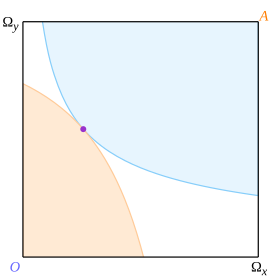
An allocation of goods is said to 'Pareto dominate' another if it is preferable for one consumer and no worse for the other. An allocation is said to be 'Pareto optimal' (or 'Pareto efficient') if no other allocation Pareto dominates it. The set of Pareto optimal allocations is known as the Pareto set (or 'efficient locus').
Consider a pair of tangential curves, one for each consumer as illustrated in Fig. 5, where the point of tangency is shown by the purple dot. Then convexity guarantees that the curves cannot intercept other than at the point of tangency, and the box is accordingly divided into 3 regions. The pale blue area is preferable to the point of tangency for Octavio but worse for Abby; the pale orange area is preferable for Abby but worse for Octavio; and the white area is worse for both. Similar considerations apply to the boundaries. It follows that the point of tangency is Pareto optimal.

Thus the Pareto set is the locus of points of tangency of the curves. This is a line connecting Octavio's origin (O) to Abby's (A). An example is shown in Fig. 6, where the purple line is the Pareto set corresponding to the indifference curves for the two consumers.
The vocabulary used to describe different objects which are part of the Edgeworth box diverges. The entire Pareto set is sometimes called the contract curve, while Mas-Colell et al. restrict the definition of the contract curve to only those points on the Pareto set which make both Abby and Octavio at least as well off as they are at their initial endowment. Other authors who have a more game theoretical bent, such as Martin Osborne and Ariel Rubinstein,[13] use the term core for the section of the Pareto set which is at least as good for each consumer as the initial endowment.
Since the Pareto set is the set of points where the consumers' indifference curves are tangential, it is also the set of points where each consumer's marginal rate of substitution is equal to that of the other person.[14]
The first fundamental theorem of welfare economics
[edit]We have seen that the points of tangency of indifference curves are the Pareto optima, but we also saw previously that the economic equilibria are those points at which indifference curves are tangential to a common price line. It follows that the equilibria are precisely the Pareto optima.
This argument applies with one restriction even if the curves are undifferentiable or if the equilibrium is on the boundary. The condition for equilibrium is that no further exchange will take place, and the condition for no further exchange to take place is that there is no direction of motion which benefits one consumer without harming the other; and this is equivalent to the definition of a Pareto optimum.[15]
The restriction is that equilibrium implies that no local improvement can be made – in other words, that the point is 'locally' Pareto optimal. But Pareto optimality is nowadays considered global by definition.[16] Thus if the nature of the indifference curves allows non-global optima to arise (as cannot happen if they are convex), then it is possible for equilibria not to be Pareto optimal.
Perfect competition is not a precondition for the theorem. So long as the consumers are free to exchange, and will continue to do so until no mutually acceptable exchange is available, equilibrium will be reached and will be (at least 'locally') Pareto optimal.[17]
The second fundamental theorem of welfare economics
[edit]
Now consider an economy in which the consumers have endowments ω as shown in Fig. 7. Left to itself a free market will take them to ω'. But suppose that some other position in the box – say α' – is considered socially preferable. We can assume that the socially desired position is Pareto optimal.
We may think of the price lines (shown as dashed in the diagram) as corresponding to different distributions of real income, and movement along them as reallocation of resources while incomes remain fixed.
Then in order to reposition society at the desired point α' it is not necessary for the government to redistribute resources in such a way that Octavio holds (α'x,α'y) and Abby holds the complement: it is sufficient to reallocate resources to take the economy to any point (say α) on the price line through α', and then leave the market to find its own equilibrium. Indeed, so long as the government recognises a desirable distribution of income it does not need to have any idea of the optimal allocation of resources.
In a statement for a more general economy, the theorem would be taken as saying that α' can be reached by a monetary transfer followed by the free play of market exchange; but money is absent from the Edgeworth box.
The second fundamental theorem does not provide a blueprint for righting society's ills. The government may decide to reallocate resources between Octavio and Abby, moving them from ω to α in advance of the day's trading; and in consequence whoever loses out may decide to take less to market the next day. The second fundamental theorem takes no account of the distortions introduced by the reallocation.[18]
Offer curves
[edit]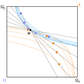
Offer curves provide a means of finding points of equilibrium, and are also useful for investigating their existence and uniqueness.
Two such curves, one for each consumer and both depending on the endowment, can be drawn in the box. We pivot the budget line about ω and trace the two consumers' most favoured points along the line as shown by the coloured dots in Fig. 8. These are points at which the line is tangential to their own indifference curves.

The locus of a consumer's most favoured points is his or her offer curve. Fig. 9 shows Octavio's offer curve as dark blue and Abby's as brown. They meet at the point ω' and the equilibrium budget line (drawn in grey) is the one passing through this point. The indifference curves through ω' for the two consumers are shown in paler colours.
An offer curve necessarily passes through the endowment point ω. If we take Abby as an example, we note that one of her indifference curves must pass through ω and that a budget line can be chosen to have the same gradient as the indifference curve here, making ω a most favoured point for this line.
In consequence the two consumers' offer curves necessarily intersect at ω; but the property which makes this happen is that ω is the only possible point of intersection consistent with budget lines of differing gradient, and that therefore it doesn't necessarily constitute an equilibrium.
Any intersection of offer curves at a point other than ω determines a stable equilibrium. If the two offer curves are tangential at the endowment point, then this point is indeed an equilibrium and their common tangent is the corresponding budget line.[19]
Terminology for offer curves
[edit]Offer curves were first used by Vilfredo Pareto – see his Manuale/Manuel Chap. III, §97. He called them 'exchange curves' (linee dei baratti / lignes des échanges), and his name for Octavio's preferred allocation along a budget line was his 'equilibrium point'.
This preferred allocation is sometimes nowadays referred to as Octavio's 'demand', which constitutes an asymmetric description of a symmetric fact. An allocation determines Abby's holding as much as Octavio's, and is therefore as much a supply as a demand.
Offre is French for 'supply', so calling an offer curve a locus of demands amounts to calling a supply curve a locus of demands.
Uniqueness of equilibria
[edit]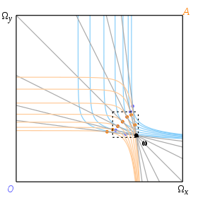

It might be supposed from economic considerations that if a shared tangent exists through a given endowment, and if the indifference curves are not pathological in their shape, then the point of tangency will be unique. This turns out not to be true. Conditions for uniqueness of equilibrium have been the subject of extensive research: see General equilibrium theory.
Figs. 9 and 10 illustrate an example from Mas-Colell et al. in which three distinct equilibria correspond to the endowment point ω. The indifference curves are:
(Octavio)
(Abby).
The indifference curves fill the box but are only shown when tangential to some representative budget lines. The offer curves, drawn in Fig. 11, cross at three points shown by large grey dots and corresponding to exchange rates of 1⁄2, 1 and 2.
Generalisations
[edit]Early examinations of the properties of equilibrium were based on an implicit definition as tangency, and convexity seems to have been implicitly assumed.[20] There was no doubt that equilibrium would be reached: gradient ascent would lead to it. But the results lacked generality.
Boundary equilibria and non-differentiable curves
[edit]
Kenneth Arrow and Gérard Debreu published papers independently in 1951 drawing attention to limitations in the calculus proofs of equilibrium theorems.[21] Arrow specifically mentioned the difficulty caused by equilibria on the boundary, and Debreu the problem of non-differentiable indifference curves.
Without aiming for exhaustive coverage it is easy to see in intuitive terms how to extend our methods to apply to these cases. We need to broaden the concept of a tangent to include any line which touches the curve: a tangent in the etymological sense rather than that of the differential calculus. In the example of Fig. 12 there is an arc of legal price lines through a point of contact, each touching indifference curves without cutting them inside the box, and accordingly there is a range of possible equilibria for a given endowment.
Competitive equilibrium
[edit]The equilibria of Fig. 12 are not points at which curves are true tangents to each other. They do however have a property which generalises the definition in terms of tangents, which is that the two curves can be locally separated by a straight line.
Arrow and Debreu defined equilibrium in the same way as each other in their (independent) papers of 1951 without providing any source or rationale for their definition. They retained their definition in their joint paper (on the existence of equilibrium) of 1954.[22] The new definition required a change of mathematical technique from the differential calculus to convex set theory.
Their definition in effect was this: an equilibrium attainable from an endowment ω consists of an allocation x and a budget line through x and ω such that there is no point along the line which either consumer (strictly) prefers to x. A pair comprising an allocation and a line which satisfies this property is known as a 'Walrasian' or 'competitive' equilibrium.
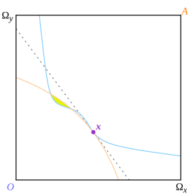
The budget line of this definition is a line which separates the indifference curves of the two consumers, but it does so globally rather than locally. Arrow and Debreu do not explain why they require global separation, which may have made their proofs easier but can be seen to have unexpected consequences. In Fig. 13 the point x is a point of tangency which is also a point at which indifference curves are locally separated by the dashed price line; but since they are not globally separated the point is not an equilibrium according to Arrow and Debreu's definition.

In Fig. 14 the point x is a Pareto optimum which does not satisfy the definition of competitive equilibrium. The question of whether the economy would settle at such a point is quite separate from whether it satisfies a given definition of equilibrium; evidently in this case it would indeed settle there.
Arrow and Debreu always included the convexity of indifference curves amongst their 'assumptions'. The term 'assumptions' is a vague one which might refer to a presupposition underlying definitions as well as theorems, or to a premise which is needed only for the latter. Given that their definition does not include all equilibria which may exist when curves may be non-convex, it is possible that they meant the assumption of convexity in the former sense. Whether or not this is so, the definition has been widely adopted without any restriction of domain.
It has sometimes been found that results can be derived under their definition without assuming convexity in the proof (the first fundamental theorem of welfare economics being an example).
Existence of competitive equilibrium
[edit]In some economies there will be no resting point reachable from a given endowment by exchange at uniform prices; hence no resting point exists satisfying the definition of competitive equilibrium. Families of curves of the pattern of Fig. 14 are an example of this.
The fundamental theorems of welfare economics
[edit]With equilibrium defined as 'competitive equilibrium', the first fundamental theorem can be proved even if indifference curves need not be convex: any competitive equilibrium is (globally) Pareto optimal. However the proof is no longer obvious, and the reader is referred to the article on Fundamental theorems of welfare economics.
The same result would not have been considered to hold (with non-convex indifference curves) under the tangency definition of equilibrium. The point x of Fig. 13 would have been considered an equilibrium which was not (globally) optimal since the yellow region Pareto dominates it.
It does not follow that the result has been strengthened since the attainability of equilibrium has been rendered doubtful. In Fig. 13 the point x may not be a 'competitive equilibrium', but the economy can get stuck there preventing it from reaching the 'true' (and Pareto optimal) equilibrium in the yellow region.
It was always considered essential to the first welfare theorem that equilibrium would actually be attained. Lerner's interpretation of the theorem was that "Fortunately the optimum allocation of goods can be reached automatically".[23] However nothing can guarantee that a global optimum will be attained when local optima are present. If the concept of equilibrium includes local optima such as x, then equilibrium may be attainable but sub-optimal; if such points are excluded, then equilibrium may be optimal but unattainable.
The differences caused by non-convexity become more deep-rooted when we look at the second fundamental theorem. Not every Pareto optimum is a competitive equilibrium (though it may still be a resting place for the economy). Consequently the theorem needs either to be given convexity of preferences as a premise, or else to be stated in such a way that 'equilibrium' is not understood as 'competitive equilibrium' as defined above.
Notes
[edit]- ^ John Creedy, 2008. "Francis Ysidro Edgeworth (1845–1926)", The New Palgrave Dictionary of Economics, 2nd Edition. Abstract.
- ^ John F. Nash, Jr., 1950. "The Bargaining Problem," Econometrica, 18(2), pp. 155-162.
- ^ Roberto Serrano, 2008. "bargaining," The New Palgrave Dictionary of Economics, 2nd Edition. Abstract.
- ^ Schotter, Andrew (2008), Microeconomics: A Modern Approach, Cengage Learning, p. 524, ISBN 978-0-324-31584-4
- ^ Lluís Barbé (2010), Francis Ysidro Edgeworth: a portrait with family and friends, Edward Elgar Publishing, p. 12, ISBN 978-1-84844-716-5
- ^ Humphrey, Thomas M. "Early History of the Box Diagram" (PDF). Economic Quarterly. Retrieved 30 October 2016.
- ^ L. Walras, 'Éléments d'Économie Politique Pure, ou Théorie de la Richesse Sociale' (1874).
- ^ V. Pareto, Manuale/Manuel (1906/9).
- ^ A. Wald, 'Über einige Gleichungssysteme der mathematischen Ökonomie' (1936), tr. as "On some Systems of Equations of Mathematical Economics" (1951).
- ^ P. Samuelson, "Foundations of Economic Analysis" (1947).
- ^ K. Arrow and G. Debreu, "Existence of an Equilibrium for a Competitive Economy" (1954).
- ^ See Pareto, Manuale/Manuel, Chap. III, §170. Notice that Pareto is careful not to say that constant prices are general, merely that they are the commonest and most important case.
- ^ Osborne, Martin J.; Rubinstein, Ariel (1994). A Course in Game Theory. Cambridge: MIT Press. ISBN 0-262-65040-1.
- ^ The Cobb-Douglas αs for the illustrations are 0·35 (Octavio) and 0·65 (Abby).
- ^ See K. Wicksell, "Lectures on Political Economy" I (1906), Eng. tr. (1934), pp. 82 f.
- ^ Pareto himself defined it as a local property. Manuale/Manuel Chap III, §22.
- ^ See Paul Samuelson, 'Foundations of Economic Analysis' (1947), p. 204.
- ^ See the discussion on pp. 556 f. of Mas-Colell et al.
- ^ This account is based on Section 15.B of Mas-Colell et al. The illustration is their Example 15.B.1 with its Cobb-Douglas α set equal to 0·275.
- ^ Oscar Lange, "The Foundations of Welfare Economics" (1942).
- ^ K. Arrow, "An Extension of the Basic Theorems of Classical Welfare Economics" (1951); G. Debreu, "The Coefficient of Resource Utilization" (1951).
- ^ K. Arrow and G. Debreu, "Existence of an Equilibrium for a Competitive Economy" (1954).
- ^ A. Lerner, "The Economics of Control" (1944), p. 15.
References
[edit]- Mas-Colell, Andreu; Whinston, Michael D.; Jerry R. Green (1995). Microeconomic Theory. New York: Oxford University Press. ISBN 0-19-507340-1.
- Vilfredo Pareto, Manuale di Economia Politica con una Introduzione alla Scienza Sociale (1906) / Manuel d'Économie Politique (1909) (effectively a second edition of the Italian version), Eng. tr. (of the French) as "Manual of Political Economy" (1971). The Italian text is available online at https://archive.org/details/manualedieconomi00pareuoft.


